Chaos and Fractals in Financial Markets

The French Gambler and the Pollen Grains

In 1827 an English botanist, Robert Brown got his hands on some new technology: a microscope "made for me by Mr. Dolland, . . . of which the three lenses that I have generally used, are of a 40^th, 60^th, and 70^th of an inch focus."

Right away, Brown noticed how pollen grains suspended in water jiggled around in a furious, but random, fashion.

To see what Brown saw under his microscope, make sure that Java is enabled on your web browser, and then click here.

What was going on was a puzzle. Many people wondered: Were these tiny bits of organic matter somehow alive? Luckily, Hollywood wasn’t around at the time, or John Carpenter might have made his wonderful horror film They Live! about pollen grains rather than about the infiltration of society by liberal control-freaks.

Robert Brown himself said he didn’t think the movement had anything to do with tiny currents in the water, nor was it produced by evaporation. He explained his observations in the following terms:

"That extremely minute particles of solid matter, whether obtained from organic or inorganic substances, when suspended in pure water, or in some other aqueous fluids, exhibit motions for which I am unable to account, and from which their irregularity and seeming independence resemble in a remarkable degree the less rapid motions of some of the simplest animalcules of infusions. That the smallest moving particles observed, and which I have termed Active Molecules, appear to be spherical, or nearly so, and to be between 1-20,0000dth and 1-30,000dth of an inch in diameter; and that other particles of considerably greater and various size, and either of similar or of very different figure, also present analogous motions in like circumstances.

"I have formerly stated my belief that these motions of the particles neither arose from currents in the fluid containing them, nor depended on that intestine motion which may be supposed to accompany its evaporation."[1]

Brown noted that others before him had made similar observations in special cases. For example, a Dr. James Drummond had observed this fishy, erratic motion in fish eyes:

"In 1814 Dr. James Drummond, of Belfast, published in the 7^th Volume of the Transactions of the Royal Society of Edinburgh, a valuable Paper, entitled ‘On certain Appearances observed in the Dissection of the Eyes of Fishes.’

"In this Essay, which I regret I was entirely unacquainted with when I printed the account of my Observations, the author gives an account of the very remarkable motions of the spicula which form the silvery part of the choroid coat of the eyes of fishes."

Today, we know that this motion, called Brownian motion in honor of Robert Brown, was due to random fluctuations in the number of water molecules bombarding the pollen grains from different directions.

Experiments showed that particles moved further in a given time interval if you raised the temperature, or reduced the size of a particle, or reduced the "viscosity" [2] of the fluid. In 1905, in a celebrated treatise entitled The Theory of the Brownian Movement [3], Albert Einstein developed a mathematical description which explained Brownian motion in terms of particle size, fluid viscosity, and temperature. Later, in 1923, Norbert Wiener gave a mathematically rigorous description of what is now referred to as a "stochastic process." Since that time, Brownian motion has been called a Wiener process, as well as a "diffusion process", a "random walk", and so on.

But Einstein wasn’t the first to give a mathematical description of Brownian motion. That honor belonged to a French graduate student who loved to gamble. His name was Louis Bachelier. Like many people, he sought to combine duty with pleasure, and in 1900 in Paris presented his doctoral thesis, entitled Théorie de la spéculation.

What interested Bachelier were not pollen grains and fish eyes. Instead, he wanted to know why the prices of stocks and bonds jiggled around on the Paris bourse. He was particularly intrigued by bonds known as rentes sur l’état— perpetual bonds issued by the French government. What were the laws of this jiggle? Bachelier wondered. He thought the answer lay in the prices being bombarded by small bits of news. ("The British are coming, hammer the prices down!")

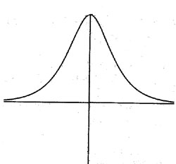
Among other things, Bachelier observed that the probability intervals into which prices fall seemed to increased or decreased with the square-root of time (T^0.5). This was a key insight.

By "probability interval" we mean a given probability for a range of prices. For example, prices might fall within a certain price range with 65 percent probability over a time period of one year. But over two years, the same price range that will occur with 65 percent probability will be larger than for one year. How much larger? Bachelier said the change in the price range was proportional to the square root of time.

Let P be the current price. After a time T, the prices will (with a given probability) fall in the range

(P –a T^0.5, P + a T^0.5), for some constant a.

For example, if T represents one year (T=1), then the last equation simplifies to

(P –a , P + a), for some constant a.

The price variation over two years (T=2) would be

a T^0.5 = a(2)^0.5 = 1.4142 a

or 1.4142 times the variation over one year. By contrast, the variation over a half-year (T=0.5) would be

a T^0.5 = a(0.5) ^0.5 = .7071 a

or about 71 percent of the variation over a full year. That is, after 0.5 years, the price (with a given probability) would be in the range

(P –.7071a , P + .7071a ).

Here the constant a has to be determined, but one supposes it will be different for different types of prices: a may be bigger for silver prices than for gold prices, for example. It may be bigger for a share of Yahoo stock than for a share of IBM.

The range of prices for a given probability, then, depends on the constant a, and on the square root of time (T^0.5). This was Bachelier’s insight.

Now, to be sure, Bachelier made a financial mistake. Remember (from Part 1 of this series) that in finance we always take logarithms of prices. This is for many reasons. Most changes in most economic variables are proportional to their current level. For example, it is plausible to think that the variation in gold prices is proportional to the level of gold prices: $800 dollar gold varies in greater increments than does gold at $260.

The change in price, DP, as a proportion of the current price P, can be written as:

DP/P .

But this is approximately the same as the change in the log of the price:

DP/P » D (log P) .

What this means is that Bachelier should have written his equation:

(log P –a T^0.5, log P + a T^0.5), for some constant a.

However, keep in mind that Bachelier was making innovations in both finance and in the mathematical theory of Brownian motion, so he had a hard enough time getting across the basic idea, without worrying about fleshing out all the correct details for a non-existent reading audience. And, to be sure, almost no one read Bachelier’s PhD thesis, except the celebrated mathematician Henri Poincaré, one of his instructors.

The range of prices for a given probability, then, depends on the constant a, and on the square root of time (T^0.5), as well as the current price level P.

To see why this is true, note that the probability range for the log of the price

(log P –a T^0.5, log P + a T^0.5)

translates into a probability range for the price itself as

( P exp(- a T^0.5), P exp( a T^0.5 ) ) .

(Here "exp" means exponential, remember? For example, exp(-.7) = e ^-.7 = 2.718281^-.7 = .4966. )

Rather than adding a plus or minus something to the current price P, we multiply something by the current price P. So the answer depends on the level of P. For a half-year (T=0.5), instead of

(P –.7071a , P + .7071a )

we get

( P exp(- .7071 a ), P exp( .7071 a ) ) .

The first interval has a constant width of 1.4142 a, no matter what the level of P (because P + .7071 a - (P -.7071 a) = 1.4142 a). But the width of the second interval varies as P varies. If we double the price P, the width of the interval doubles also.

Bachelier allowed the price range to depend on the constant a and on the square root of time (T^0.5), but omitted the requirement that the range should also depend on the current price level P.

The difference in the two approaches is that if price increments (DP) are independent, and have a finite variance, then the price P has a normal (Gaussian distribution). But if increments in the log of the price (D log P) are independent, and have a finite variance, then the price P has a lognormal distribution.

Here is a picture of a normal or Gaussian distribution:

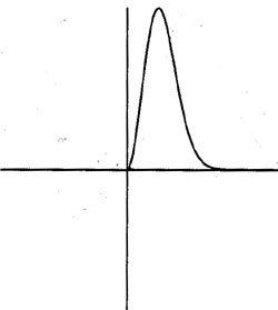
The left-hand tail never becomes zero. No matter where we center the distribution (place the mean), there is always positive probability of negative numbers.

Here is a picture of a lognormal distribution:

The left-hand tail of a lognormal distribution becomes zero at zero. No matter where we center the distribution (place the mean), there is zero probability of negative numbers.

A lognormal distribution assigns zero probability to negative prices. This makes us happy because most businesses don’t charge negative prices. (However, US Treasury bills paid negative interest rates on certain occasions in the 1930s.) But a normal distribution assigns positive probability to negative prices. We don’t want that.

So, at this point, we have seen Bachelier’s key insight that probability intervals for prices change proportional to the square root of time (that is, the probability interval around the current price P changes by a T^0.5), and have modified it slightly to say that probability intervals for the log of prices change proportional to the square root of time (that is, the probability interval around log P changes by a T^0.5).

Now we are going to take a break from price distributions, and pursue the question of how we measure things. How we measure length, area, volume, or time. (This will lead us from Bachelier to Mandelbrot.)

Usually, when we measure things, we use everyday dimensions (or at least the ones we are familiar with from elementary plain geometry). A point has zero dimension. A line has one dimension. A plane or a square has two dimensions. A cube has three dimensions. These basic, common-sense type dimensions are sometimes referred to as topological dimensions.

We say a room is so-many "square feet" in size. In this case, we are using the two-dimensional concept of area. We say land is so-many "acres" in size. Here, again, we are using a two-dimensional concept of area, but with different units (an "acre" being 43,560 "square feet"). We say a tank holds so-many "gallons". Here we are using a measure of volume (a "gallon" being 231 "cubic inches" in the U.S., or .1337 "cubic feet").

Suppose you have a room that is 10 feet by 10 feet, or 100 square feet. How much carpet does it take to cover the room? Well, you say, a 100 square feet of carpet, of course. And that is true, for ordinary carpet.

Let’s take a square and divide it into smaller pieces. Let’s divide each side by 10:

We get 100 pieces. That is, if we divide by a scale factor of 10, we get 100 smaller squares, all of which look like the big square. If we multiply any one of the smaller squares by 10, we get the original big square.

Let’s calculate a dimension for this square. We use the same formula as we used for the Sierpinski carpet:

N = r^D .

Taking logs, we have log N = D log r, or D = log N/ log r.

We have N = 100 pieces, and r = 10, so we get the dimension D as

D = log(100)/log(10) = 2.

(We are using "log" to mean the natural log, but notice for this calculation, which involves the ratio of two logs, that it doesn’t matter what base we use. You can use logs to the base 10, if you wish, and do the calculation in your head.)

We called the dimension D calculated in this way (namely, by comparing the number of similar objects N we got at different scales to the scale factor r) a Hausdorff dimension. In this case, the Hausdorff dimension 2 is the same as the ordinary or topological dimension 2.

So, in any case, the dimension is 2, just as you suspected all along. But suppose you covered the floor with Sierpinski carpet. How much carpet do you need then?

We saw (in Part 1) that the Sierpinski carpet had a Hausdorff dimension D = 1.8927… A Sierpinski carpet which is 10 feet on each side would only have N = 10^1.8927 = 78.12 square feet of material in it.

Why doesn’t a Sierpinski carpet with 10 feet on each side take 100 square feet of material? Because the Sierpinski carpet has holes in it, of course.

Remember than when we divided the side of a Sierpinski carpet by 3, we got only 8 copies of the original because we threw out the center square. So it had a Hausdorff dimension of D = log 8/ log 3 = 1.8927. Then we divided each of the 8 copies by 3 again , threw out the center squares once more, leaving 64 copies of the original. Dividing by 3 twice is the same as dividing by 9, so, recalculating our dimension, we get D = log 64/ log 9 = 1.8927.

An ordinary carpet has a Hausdorff dimension of 2 and a topological (ordinary) dimension of 2. A Sierpinski carpet has a Hausdorff dimension of 1.8927 and a topological dimension of 2. [4]

Benoit Mandelbrot defined a fractal as an object whose Hausdorff dimension is different from its topological dimension. So a Sierpinski carpet is a fractal. An ordinary carpet isn’t.

Fractals are cheap and sexy. A Sierpinski carpet needs only 78.12 square feet of material to cover 100 square feet of floor space. Needing less material, a Sierpinski carpet costs less. Sure it has holes in it. But the holes form a really neat pattern. So a Sierpinski carpet is sexy. Cheap and sexy. You can’t beat that.

Let’s see if we have this fractal stuff straight. Let’s look at the first known fractal, created in 1870 by the mathematical troublemaker George Cantor.

Remember that we create a fractal by forming similar patterns at different scales, as we did with the Sierpinski carpet. It’s a holey endeavor. In order to get a carpet whose Hausdorff dimension was less than 2, we created a pattern of holes in the carpet. So we ended up with an object whose Hausdorff dimension D (which compares the number N of different, but similar, objects at different scales r, N = r^D ) was more than 1 but less than 2. That made the Sierpinski carpet a fractal, because its Hausdorff dimension was different from its topological dimension.

What George Cantor created was an object whose dimension was more than 0 but less than 1. That is, a holey object that was more than a point (with 0 dimensions) but less than a line (with 1 dimension). It’s called Cantor dust. When the Cantor wind blows, the dust gets in your lungs and you can’t breathe.

To create Cantor dust, draw a line and cut out the middle third:

0________________________________________________________1

0__________________1/3               2/3_________________1

Now cut out the middle thirds of each of the two remaining pieces:

0____1/9   2/9____ 1/3               2/3____7/9  8/9 ____1

Now cut out the middle thirds of each of the remaining four pieces, and proceed in this manner for an infinite number of steps, as indicated in the following graphic.

What's left over after all the cutting is Cantor dust.

At each step we changed scale by r = 3, because we divided each remaining part into 3 pieces. (Each of these pieces had 1/3 the length of the original part.) Then we threw away the middle piece. (That’s how we created the holes.) That left 2 pieces. At the next step there were 4 pieces, then 8, and so on. At each step the number of pieces increased by a factor of N = 2. Thus the Hausdorff dimension for Cantor dust is:

D = log 2 / log 3 = .6309.

Is Cantor dust a fractal? Yes, as long as the topological dimension is different from .6309, which it surely is.

But—what is the topological dimension of Cantor dust? We can answer this by seeing how much of the original line (with length 1) we cut out in the process of making holes.

At the first step we cut out the middle third, or a length of 1/3. The next step we cut out the middle thirds of the two remaining pieces, or a length of 2(1/3)(1/3). And so on. The total length cut out is then:

1/3 + 2(1/3²) + 4(1/3³) + 8(1/3⁴) + . . . = 1.

We cut out all of the length of the line (even though we left an infinite number of points), so the Cantor dust that's left over has length zero. Its topological dimension is zero. Cantor dust is a fractal with a Hausdorff dimension of .6309 and a topological dimension of 0.

Now, the subhead refers to Cantor dust as "history’s first fractal". That a little anthropocentric. Because nature has been creating fractals for millions of years. In fact, most things in nature are not circles, squares, and lines. Instead they are fractals, and the creation of these fractals are usually determined by chaos equations. Chaos and fractal beauty are built into the nature of reality. Get used to it.

Today, there are roughly of order 10³ recognized fractal systems in nature, though a decade ago when Mandelbrot's classic Fractal Geometry of Nature was written, many of these systems were not known to be fractal. [5]

So far we’ve seen that measuring things is a complicated business. Not every length can be measured with a tape measure, nor the square footage of material in every carpet measured by squaring the side of the carpet.

Many things in life are fractal, and follow power laws just like the D of the Hausdorff dimension. For example, the "loudness" L of noise as heard by most humans is proportional to the sound intensity I raised to the fractional power 0.3:

L = a I^0.3 .

Doubling the loudness at a rock concert requires increasing the power output by a factor of ten, because

a (10 I)^0.3 = 2 a I^0.3 = 2 L .

In financial markets, another subjective domain, "time" is fractal. Time does not always move with the rhythms of a pendulum. Sometimes time is less than that. In fact, we’ve already encounted fractal time with the Bachelier process, where the log of probability moved according to

a T^0.5 .

Bachelier observed that if the time interval was multiplied by 4, the probability interval only increased by 2. In other words, at a scale of r = 4, the number N of similar probability units was N = 2. So the Hausdorff dimension for time was:

D = log N/ log r = log 2/ log 4 = 0.5 .

In going from Bachelier to Mandelbrot, then, the innovation is not in the observation that time is fractal: that was Bachelier’s contribution. Instead the question is: What is the correct fractal dimension for time in speculative markets? Is the Hausdorff dimension really D = 0.5, or does it take other values? And if the Hausdorff dimension of time takes other values, what’s the big deal, anyway?

The way in which Mandlebrot formulated the problem provides a starting point:

Despite the fundamental importance of Bachelier's process, which has come to be called "Brownian motion," it is now obvious that it does not account for the abundant data accumulated since 1900 by empirical economists, simply because the empirical distributions of price changes are usually too "peaked" to be relative to samples from Gaussian populations. [6]

What does Mandelbrot mean by "peaked"? It’s now time for a discussion of probability.

Probability is a one-pound jar of jelly. You take the jelly and smear it all over the real line. The places where you smear more jelly have more probability, while the places where you smear less jelly have less probability. Some spots may get no jelly. They have no probability at all—their probability is zero.

The key is that you only have one pound of jelly. So if you smear more jelly (probability) at one location, you have to smear less jelly at another location.

Here is a picture of jelly smeared in the form of a bell-shaped curve:

The jelly is smeared between the horizontal (real) line all the way up to the curve, with a uniform thickness. The result is called a "standard normal distribution". ("Standard" because its mean is 0, and the standard deviation is 1.) In this picture, the point where the vertical line is and surrounding points have the jelly piled high—hence they are more probable.

As we observed previously, for the normal distribution jelly gets smeared on the real (horizontal) line all the way to plus or minus infinity. There may not be much jelly on the distant tails, but there is always some.

Now, let’s think about this bell-shaped picture. What does Mandelbrot mean by the distribution of price changes being "too peaked" to come from a normal distribution?

Does Mandelbrot’s statement make any sense? If we smear more jelly at the center of the bell curve, to make it taller, we can only do so by taking jelly from some other place. Suppose we take jelly out of the tails and intermediate parts of the distribution and pile it on the center. The distribution is now "more peaked". It is more centered in one place. It has a smaller standard deviation—or smaller dispersion around the mean. But—it could well be still normal.

So what’s with Mandelbrot, anyway? What does he mean? We’ll discover this in Part 3 of this series.

Click here to see the Answer to Problem 1 from Part 1. The material therein should be helpful in solving Problem 2.

Meanwhile, here are two new problems for eager students:

Problem 3: Suppose you create a Cantor dust using a different procedure. Draw a line. Then divide the line into 5 pieces, and throw out the second and fourth pieces. Repeat this procedure for each of the remaining pieces, and so on, for an infinite number of times. What is the fractal dimension of the Cantor dust created this way? What is its topological dimension? Did you create a new fractal?

Problem 4: Suppose we write all the numbers between 0 and 1 in ternary. (Ternary uses powers of 3, and the numbers 0, 1, 2. The ternary number .1202, for example, stands for 1 x 1/3 + 2 x 1/9 + 0 x 1/27 + 2 x 1/81.) Show the Cantor dust we created here in Part 2 (with a Hausdorff dimension of .6309) can be created by taking all numbers between 0 and 1, and eliminating those numbers whose ternary expansion contains a 1. (In other words, what is left over are all those numbers whose ternary expansions only have 0s and 2s.)

And enjoy the fractal:

[1] Robert Brown, "Additional Remarks on Active Molecules," 1829.

[2] Viscosity is a fluid’s stickiness: honey is more viscous than water, for example. "Honey don’t jiggle so much."

[3] I am using the English title of the well-known Dover reprint: Investigations on the Theory of the Brownian Movement, Edited by R. Furth, translated by A.D. Cowpter, London, 1926. The original article was in German and titled somewhat differently.

[4] I am admittingly laying a subtle trap here, because of the undefined nature of "topological dimension". This is partially clarified in the discussion of Cantor dust, and further discussed in Part 3.

[5] H. Eugene Stanley, Fractals and Multifractals, 1991

[6] Benoit Mandelbrot, "The Variation of Certain Speculative Prices," Journal of Business, 36(4), 394-419, 1963.

J. Orlin Grabbe is the author of International Financial Markets, and is an internationally recognized derivatives expert. He has recently branched out into cryptology, banking security, and digital cash. His home page is located at http://www.aci.net/kalliste/homepage.html .